

Since we’ve looked into a regular patch antenna simulation on MaxLLG, it’s time to see what one can obtain for a magnetic patch antenna. This type of antenna has appealed scientific attention due to their tunability and reconfigurability resulting from the coupling between the antenna resonant modes and the magnetic ones [1,2]. The software enables a thorough investigation of this effect with the batch feature.
The structure is similar to that of described in the case study, but the space between the radiating patch and the ground plate is filled with magnetic substance (Fig.1a) having the saturation magnetisation 4 = 1750 G, which corresponds to yittrium iron garnet (YIG). In order to limit a spectra range to lower frequencies and suppress refractions from the magnet face, the relative permittivity of both YIG and the dielectric layer is set to 2.2.
To create the 3D model, the step files from the regular patch antenna simulation are used with some modifications. The dielectric layer is recreated to have empty space beneath the patch and add there another step file for the magnet created with the following number of cells: 50x64x8. The 3D CAD Files will have the same material and dimension parameters with the updated dielectric step file and the additional magnet one (Magnetisation – 0.175, Conductivity – 0, Dielectric – 2.2). When setting Solver Parameters, the metascript file of the regular antenna simulation can be uploaded, since the excitation remains identical. One should take into account that the relative permittivity is reduced to 2.2, therefore pulse spread should be set to 100 time steps to prevent input and output signals from overlapping each other. Besides, Magnetic Parameters should be activated with the applied field and magnetic components oriented transversely to the signal propagation, e.g. along  -axis. To suppress unwanted noise specific to magnets, the damping constant is increased to 0.01.
The difference between the magnetic patch antenna and the regular one can be seen in Fig.1b, where magnetic resonances along with the main mode shift appear even at zero applied magnetic field. If we activate the field and incrementally increase it, the effect of coupling between the magnetic modes and the antenna resonance modes takes place, leading to the latter shifting toward upper frequencies. It can be easily done with the batch-feature that runs the same project multiple times in a row with a user-defined step. In this example, reflection coefficients  of the magnetic patch antenna are obtained for an applied magnetic field range from 0 to 4 kOe (80 steps) and compiled into the spectrum heatmap (Fig.1c) . It gives a clear illustration of how the main working antenna modes can be controlled. To make sure of the results, Fig.1d shows selected spectra for different magnetic field values, where the first two antenna modes are highlighted with yellow (1st mode) and red (2nd mode) circles. Looking at their field patterns (Fig.1e), it goes to prove that the magnetic patch antenna facilitates tunability.
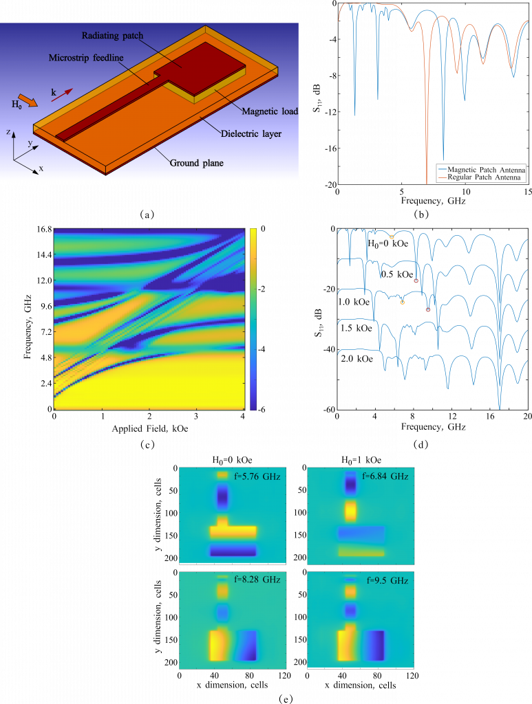
Fig. 1. a) Magnetic patch antenna schematic. b) Fourier transform of frequency-domain reflection coefficient for the regular patch antenna (orange line) and the one with YIG incorporated (blue line). c) Simulation heatmap for the magnetic antenna. d) Reflection coefficient for different values of biasing magnetic field. e) Field patterns of the  component for the first (upper) and the second (lower) modes for the two applied magnetic field values.
[1] Evmorfili A., et al., Magnetodielectric Materials in Antenna Design: Exploring the Potentials for Reconfigurability, IEEE Antennas and Propagation Magazine, 61(1), pp. 29–40, 2019.
[2] Gurevich A.G., Melkov G. A., Magnetization Oscillations and Waves, CRC Press, 1996.